2. Frames, spectrograms and features

What you will learn

• How a waveform becomes the matrix a speech model reads: windows, hops, spectra, mel filters and logarithms, with the numbers for 16 kHz audio. A Fourier transform is computed by hand on 8 samples.
• How to read a spectrogram: where silence, a vowel, a fricative, a stop release and a Mandarin tone appear, with numbers measured on two real recordings.
• Why "an 80-bin log-mel" is not one thing: eight common front ends, their defaults, and which differences a model notices. Why the mel scale and the logarithm are used.
• Which feature normalizations read the future and therefore cannot stream, and the few milliseconds of look-ahead the front end adds before any model runs.

Before you start

• Chapters: 1 (samples, sample rate, scale).
• Tools: the ssh-asr environment from code/README.md. Everything runs on a CPU.

Frames: 25 ms every 10 ms

A speech model does not read samples one by one. It reads short overlapping slices of audio called frames. The classic recipe, from Kaldi's documentation, is "typically 25 ms frames shifted by 10ms each time" (Kaldi feat.dox, lines 59-71). At 16 kHz a 25 ms window is 400 samples and the 10 ms hop between frames is 160 samples. Every recognizer in this book uses these two numbers (the vocoders of the synthesis chapters use other hops). So one second of audio becomes about 100 frames, and the running example's 160 ms chunk is 16 hops.

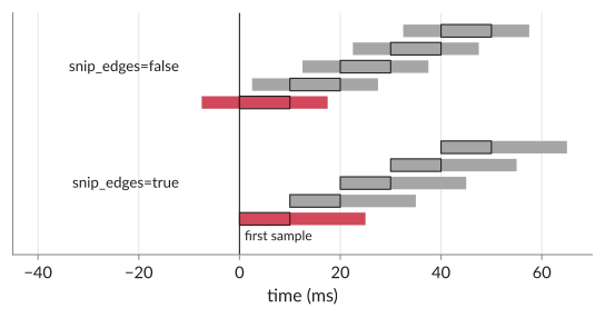
"About 100" hides a detail that matters for streaming: what happens at the edges. Kaldi has an option, snip_edges, with two behaviours (feature-window.cc, lines 28-69 and 199-214):

• snip_edges=true keeps only windows that fit entirely inside the audio: frame f starts at sample 160 f, and N samples give 1 + (N − 400) // 160 frames. One second gives 98 frames.
• snip_edges=false centers each window on its own hop: frame f covers samples 160 f − 120 to 160 f + 280, and the audio is reflected before its first sample. N samples give about N / 160 frames; one second gives 100.

The icefall and sherpa-onnx models of the CPU track use snip_edges=false; Kaldi's own default is true. Now look at where a frame ends compared with the end of its own 10 ms hop. With snip_edges=false the window ends at sample 160 f + 280, 120 samples after the hop ends at 160 f + 160: a frame is finished 7.5 ms after its hop has passed. With snip_edges=true it is 15 ms (window minus hop), and with the centered framing of NeMo and Whisper, whose window is centered on the hop's start, 2.5 ms. That is the front end's own look-ahead, and it exists before any neural network runs. Chapter 5 adds the encoder's.

What a Fourier transform computes

A frame is 400 numbers. The recognizer wants to know which frequencies those numbers contain. The discrete Fourier transform (DFT) answers that. It takes N samples and returns N numbers, one per bin. Bin k says how much of the audio repeats k times inside the N samples.

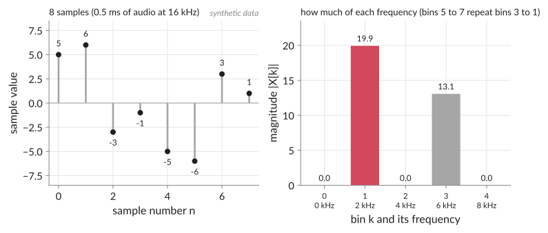
Start with 8 samples, small enough to do on paper (code/ch02_features/dft_by_hand.py, result in code/ch02_features/results/dft_by_hand.json). They are 5, 6, −3, −1, −5, −6, 3, 1. At 16 kHz they last 0.5 ms. I made them from a cosine of amplitude 5 that repeats once and a sine of amplitude 3 that repeats three times, rounded to whole numbers, so that you can see whether the transform finds them again.

The recipe for bin k has one sum. Multiply each sample x[n] by cos(2πkn/N) and by sin(2πkn/N), where n is the sample number, and add up each column over n = 0 to N − 1:

X[k] = Σ x[n] cos(2πkn/N) − i Σ x[n] sin(2πkn/N)

Here i is the imaginary unit (Python writes it 1j). It only keeps the two columns apart: the first sum is the real part of X[k], minus the second is its imaginary part.

The cosine and sine are waves that repeat k times across the N samples. If the samples contain a wave of that rhythm, its peaks meet the wave's peaks, all the products are positive, and the sum is large. If they do not, the products cancel and the sum is near 0. Here are the 8 terms for k = 1, with N = 8:

n	x[n]	cos(2πn/8)	sin(2πn/8)	x · cos	x · sin
0	5	1.000	0.000	5.000	0.000
1	6	0.707	0.707	4.243	4.243
2	−3	0.000	1.000	0.000	−3.000
3	−1	−0.707	0.707	0.707	−0.707
4	−5	−1.000	0.000	5.000	0.000
5	−6	−0.707	−0.707	4.243	4.243
6	3	0.000	−1.000	0.000	−3.000
7	1	0.707	−0.707	0.707	−0.707

The x · cos column adds up to 19.899 and the x · sin column to 1.071 (the script sums before rounding, so the rounded terms above can differ from the totals in the last digit). So X[1] = 19.899 − 1.071 i. The magnitude is the length of that pair, √(19.899² + 1.071²) = 19.928. The real and imaginary parts together also hold the phase, which the power spectrum of the next section discards; only the magnitude is kept here.

Doing this for every bin gives the table of how much of each frequency is present:

bin k	frequency	magnitude
0	0 Hz	0.000
1	2,000 Hz	19.928
2	4,000 Hz	0.000
3	6,000 Hz	13.071
4	8,000 Hz	0.000

Bins 5 to 7 are mirror copies of bins 3 to 1, as they are for any real-valued samples. Bins 0, 2 and 4 are exactly 0 because these samples are antisymmetric: x[n + 4] = −x[n] (5, 6, −3, −1, then −5, −6, 3, 1). A wave at an even bin repeats every 4 samples or less, so each pair x[n], x[n + 4] meets the same wave value with opposite signs and cancels; at odd bins the wave flips sign between the two and the pairs add. Bin 0 is the sum of the samples, 0 here, so the signal has no constant offset (the DC offset, removed in the next section). The magnitudes are 19.928 at 2 kHz and 13.071 at 6 kHz. A wave of amplitude A in a bin other than 0 and N / 2 has magnitude A · N / 2, so the amplitudes are 2 · 19.928 / 8 = 4.982 and 3.268, close to the 5 and 3 I started from (the file lists them; rounding the samples to whole numbers explains the difference). A transform that finds what was put in is a good sign. The fast Fourier transform (FFT) computes the same numbers with fewer multiplications; numpy's FFT agrees with the loop to 1.7e-14 (max_abs_difference_to_numpy_fft).

Bin spacing is the sample rate divided by the number of samples: 16,000 / 8 = 2,000 Hz here, and the last bin sits at 8 kHz, the Nyquist limit of chapter 1. The same rule gives the frame sizes of this chapter. A 400-sample frame (25 ms) gives bins 16,000 / 400 = 40 Hz apart, 201 of them. Kaldi pads the frame with zeros to 512 samples, which gives 257 bins 31.25 Hz apart. Padding adds no new information; it computes the same smooth curve at more points. A longer frame separates frequencies more finely (the bins are closer); a shorter one follows changes in the sound faster.

One frame's spectrum says which frequencies are present, not when. For when, you cut the audio into frames and compute one spectrum per frame. Stacked side by side, they are the spectrogram.

From a frame to a spectrum

Each 400-sample frame goes through the same steps. Kaldi's defaults show them all (feature-window.h, lines 54-63):

1. Dither (optional): add a tiny amount of noise so that digital silence does not produce log(0). Kaldi adds noise of standard deviation 1.0 in int16 units; most modern recipes set it to 0 at inference.
2. Remove the DC offset: subtract the frame's mean.
3. Pre-emphasis: replace each sample x[n] by x[n] − 0.97 x[n − 1], which boosts high frequencies.
4. Window: multiply by a taper that falls to zero at both ends, so the cut edges do not add false frequencies. Kaldi's default "povey" window is a Hann window raised to the power 0.85 (window(i) = pow(0.5 - 0.5*cos(a * i_fl), 0.85);, feature-window.cc, lines 124-125). NeMo and Whisper use a plain Hann window.
5. FFT: Kaldi pads the 400 samples to 512 and takes a fast Fourier transform. The result has 257 frequency bins from 0 to 8 kHz, 31.25 Hz apart. Whisper takes a 400-point FFT: 201 bins, 40 Hz apart.
6. Power: keep the squared magnitude of each bin and throw away the phase.

Steps 1 to 6, repeated every 10 ms, give a spectrogram: a picture with time across and frequency up, where dark means energy. The first figure of the section after next shows one in its middle panel.

The phase thrown away in step 6 does not come back. A spectrogram alone cannot be turned back into the exact waveform; that needs an estimate of the phase (Griffin-Lim, which torchaudio ships as torchaudio.transforms.GriffinLim) or a neural vocoder. Chapter 13 is about the vocoder.

How to read a spectrogram

A spectrogram has time across and frequency up. The shade at a point is the power in that frequency in that 25 ms frame; here dark means more power (on a decibel scale, 75 dB from lightest to darkest). Different sounds leave different shapes. The two figures below mark each shape at a position and a number measured by code/ch02_features/read_spectrogram.py (result file code/ch02_features/results/read_spectrogram.json). I chose each time range by looking at the spectrogram, and the script measures inside it; for every 10 ms frame in a range it also records the level and the centroid, so you can see that the range stays inside the sound it names (frame_level_dbfs_*, frame_centroid_hz_*). The figures use a Hann window without pre-emphasis, so levels are true levels, unlike the Kaldi front end above.

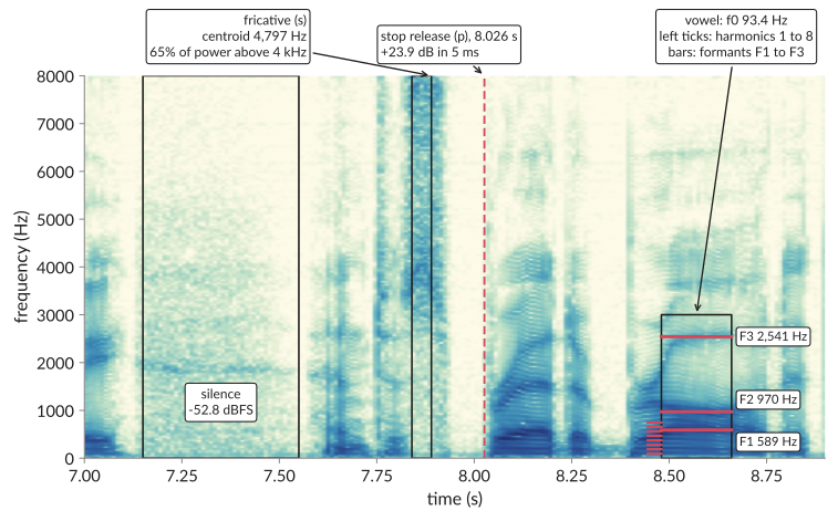
• Silence is a pale band. The pause at 7.15 to 7.55 s has a level of −52.8 dBFS (the root-mean-square level of the samples relative to the largest possible value, chapter 1); no 10 ms frame in it is louder than −48.5 dBFS. The vowel at 8.48 to 8.66 s is −23.0 dBFS, 29.8 dB higher. Silence is never zero: a recording always has a noise floor.
• A vowel (the vowel of "abroad"; I picked a steady stretch inside the word's span in the forced alignment, 8.30 to 8.74 s) shows closely spaced horizontal lines. The voice is a buzz that repeats about 93 times a second (its fundamental frequency f0, chapter 1, is 93.4 Hz), and a repeating sound has energy only at multiples of its rate, the harmonics. The measured peaks (from one 64 ms frame in the middle of the range and an 8,192-point FFT, not from the 25 ms frames of the picture, which blur neighboring harmonics) sit at 93.8, 187.5, 279.3, 373.0, 466.8, 560.5, 654.3 and 746.1 Hz, one every 93 Hz. The throat and mouth then boost some regions: the broad humps of energy are the formants. I did not read them off the humps. A 14th-order linear-prediction fit, which models the smooth curve over the harmonics, gives the median of 16 frames: F1 = 589, F2 = 970 and F3 = 2,541 Hz. Vowels differ mainly in where their formants are.
• A fricative such as the s of "spread" (7.84 to 7.89 s) is turbulent air. It shows a dark smear spread over high frequencies, with no harmonic lines (a voiced fricative such as z adds a buzz at low frequencies). I kept the range inside the run of 10 ms frames whose centroid, the power-weighted average frequency, is above 3.5 kHz (the frames starting at 7.82 through 7.90 s), with a margin. Over the range the centroid is 4,797 Hz (4,582 to 5,338 Hz frame by frame) and 65% of the power lies above 4 kHz. The vowel's centroid is 584 Hz and less than 0.1% of its power is above 4 kHz.
• A stop release is a thin vertical stripe. The lips close (a quiet gap), pressure builds, and the release is a short click with energy across many frequencies. The release of the p of "spread" is at 8.026 s, the instant inside a 110 ms search range where the 2 to 8 kHz level rises most: 23.9 dB within 5 ms.

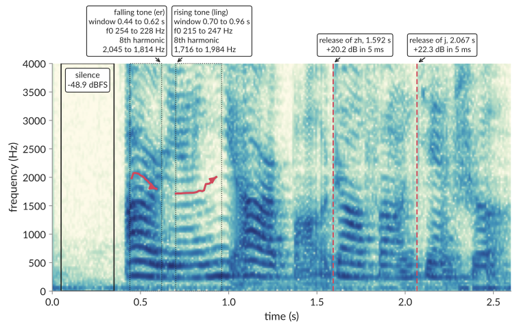
In Mandarin the pitch carries meaning, and the spectrogram shows it as slope. The numbers below are for the time windows I chose (the dotted boxes), not for whole syllables: they depend on where the window edges fall and on the script's rule that a 40 ms frame counts only if its autocorrelation peak is at least 0.6. In the first syllable, èr (fourth tone, falling), f0 goes from 254.3 Hz at the start of the window to 228.5 Hz at its end, 10% lower. In the second, líng (second tone, rising), it goes from 214.6 to 247.0 Hz, 15% higher. The harmonic at n times f0 moves n times as far, so look at a high one: the 8th falls from 2,044.9 to 1,813.8 Hz in the first window and rises from 1,716.1 to 1,983.7 Hz in the second (red lines). Every harmonic leans the same way, but on this linear axis the higher the harmonic the steeper its slope, so a tone appears as a fan of lines that spread apart upward, not as parallel lines. This is a different speaker and a different utterance from the English one (and from chapter 1's examples), and the voice is higher: f0 between 214.6 and 254.3 Hz in these two windows against 93.4 Hz, so the harmonics are spaced 2.3 to 2.7 times wider. The releases of zh in zhàng (1.592 s, +20.2 dB) and j in jiàn (2.067 s, +22.3 dB; both are affricates, a stop followed by a fricative) are the stripes at the starts of those syllables. I matched syllables to times by counting through the transcript; the measurements do not depend on that.

With this you can read what a front end gives a model. The model gets one column of numbers per 10 ms, and what separates the sounds above are exactly these patterns: level, energy at high or low frequencies, lines or no lines, slopes.

Mel filters and the logarithm

257 bins are more detail than a recognizer needs, and they are spaced evenly, while hearing is not: the difference between 200 and 300 Hz is obvious, between 7,200 and 7,300 Hz it is not. So the bins are pooled by a mel filterbank: a set of overlapping triangular filters, narrow at low frequencies and wide at high ones. Each filter sums the power under its triangle into one number. Most streaming models in this book use 80 filters; Kaldi's old default is 23 (feature-fbank.h, lines 50-60); Whisper large-v3 (config.json, line 42) and Nemotron 3.5 ASR (code/ch02_features/results/model_frontends.json) use 128.

Finally, take the logarithm of each filter's output. Loudness is heard roughly logarithmically, and the logarithm turns a gain applied to the whole signal into a constant added to every value. The result, 80 numbers every 10 ms, is the log-mel feature (also called fbank), the bottom panel below.

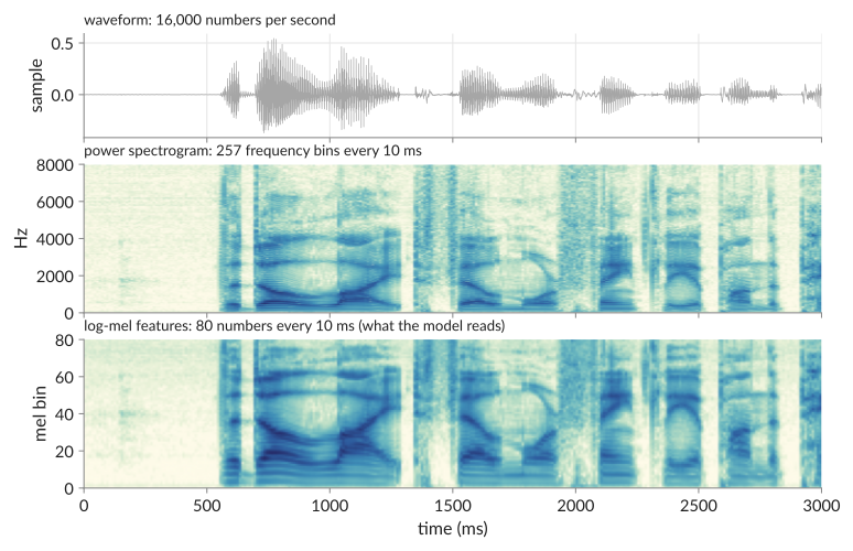
Two details of this last step differ between toolkits, and both change every number:

• Which mel scale. The HTK scale is 2595 log₁₀(1 + f/700); Kaldi writes the same curve as 1127 ln(1 + f/700). The Slaney scale is linear below 1 kHz and logarithmic above (librosa convert.py, lines 1211-1224). The two scales also use different units (at 1 kHz the HTK scale gives 1,000 and the Slaney scale 15), so their values cannot be compared, only the filter positions they produce. The curves have similar shapes, so the filters land in similar places, but not identical ones, and Slaney filters are also normalized to equal area.
• Which logarithm. Kaldi, lhotse and NeMo use the natural logarithm; Whisper uses log₁₀; a "dB" feature is 10 log₁₀. The same power gives values that differ by a factor of 2.3 between the natural logarithm and log₁₀, and by 4.3 between the natural logarithm and the dB form.

Why the mel scale and why the logarithm: the numbers

All numbers in this subsection are in code/ch02_features/results/mel_numbers.json, produced by code/ch02_features/mel_numbers.py with the CPU track's front end (80 filters, 20 to 7,600 Hz, 512-point FFT) on LibriSpeech test-clean 1089-134686-0006.

The mel scale. With the formula the code uses, 1127 ln(1 + f / 700), 500 Hz is 607.4 mel, 1,000 Hz is 1,000.0, 2,000 Hz is 1,521.4, 4,000 Hz is 2,146.1 and 8,000 Hz is 2,840.0. The scale bends. A 100 Hz step from 200 to 300 Hz is 118.7 mel. The same 100 Hz step from 7,200 to 7,300 Hz is 14.2 mel, 8.4 times smaller. The filters are spaced evenly in mel, so they crowd at low frequencies: 28 of the 80 have their center below 1 kHz, 34 between 1 and 4 kHz and 18 at or above 4 kHz. The FFT has 257 bins; 32 are below 1 kHz and 129 are at or above 4 kHz. So the lowest 1 kHz gets 28 numbers for 32 bins (the first filter is 44.8 Hz wide and covers 2 bins), while the top half of the spectrum is pooled into 18 numbers (the last filter is 486.2 Hz wide and covers 16 bins). So the mel filterbank gives fine resolution at low frequencies and coarse resolution at high ones. In the vowel above all three measured formants lie below 2.6 kHz and the harmonics are visible below 1 kHz, so that is where the detail goes; the fricative above has its energy above 4 kHz, where the 18 wide filters still capture it as a level but not as fine structure.

The logarithm. Take the sum of the 80 filter outputs of each frame as its energy. In this 10.6 s utterance (1,056 frames) the loudest frame, at 0.76 s, has energy 117.39. The quietest, at 10.15 s, has 0.00084. The loudest is 139,332 times the quietest. After the natural logarithm the two frames are 4.766 and −7.079: a span of 11.845 units. A network that reads the raw energies sees one huge number and many tiny ones; after the logarithm it sees numbers of the same order.

The second reason is gain. I halved the amplitude of the whole utterance. Every raw value became 0.25 of what it was (power goes with the square). Every log value moved by the same constant, −1.386 = 2 ln 0.5, over the 83,647 values compared (833 values at the floor were left out because they do not move: Kaldi replaces any filter output below float32's machine epsilon, 1.2e-7, by that value before the logarithm). A louder or quieter microphone therefore adds a constant to the features, which a normalizer can remove, and it does not change their shape. The next section is about which normalizers can run while the audio is still arriving.

Log-mel and MFCC. An MFCC takes the log-mel values of a frame and applies a discrete cosine transform, keeping only the first few outputs, for example 13 from 23 bins (Kaldi's feature documentation, feat.dox, lines 68-72). The models in this book skip that last step and read the log-mel values directly. Whisper's paper describes "an 80-channel log-magnitude Mel spectrogram" computed on 25 ms windows with a 10 ms stride (arXiv:2212.04356, Sec. 2.2), and the sherpa-onnx and NeMo streaming front ends in the table below also end with the logarithm.

Same name, different numbers

Here are eight front ends that all compute "a log-mel spectrogram of 16 kHz speech", with their shipped defaults. Each cell comes from the code cited in this chapter's sources.

Front end	Window / hop	FFT	Window type	Mel bins, scale	Log	Pre-emph.	Dither	Edges	Input scale
Kaldi compute-fbank-feats	25 / 10 ms	512	povey	23, HTK	ln	0.97	1.0	snip	int16 range
torchaudio compliance.kaldi.fbank	25 / 10 ms	512	povey	23, HTK	ln	0.97	0.0	snip	int16 range
lhotse Fbank (icefall training)	25 / 10 ms	512	povey	80, HTK, 20 to 7,600 Hz	ln	0.97	0.0	no snip	−1 to 1
sherpa-onnx (CPU track)	25 / 10 ms	512	povey	80, HTK, 20 to 7,600 Hz	ln	0.97	0.0	no snip	−1 to 1
NeMo streaming recipe (GPU track)	25 / 10 ms	512	Hann	80, Slaney	ln(x + 2⁻²⁴)	0.97	10⁻⁵, training only	centered	−1 to 1
Whisper	25 / 10 ms	400	Hann	80 or 128, Slaney	log₁₀, then clamp and rescale	none	none	centered, 30 s	−1 to 1
librosa melspectrogram	2,048 / 512 samples, at 22,050 Hz	2,048	Hann	128, Slaney	none	none	none	centered	−1 to 1
torchaudio MelSpectrogram	400 / 200 samples	400	Hann	128, HTK	none	none	none	centered	−1 to 1

Sources for the rows, in order: Kaldi feature-window.h, feature-fbank.h, mel-computations.h; torchaudio compliance/kaldi.py lines 514-543; lhotse features/kaldi/extractors.py lines 24-43 and icefall compute_fbank_librispeech.py; sherpa-onnx features.h lines 18-61; NeMo fastconformer_transducer_bpe_streaming.yaml lines 62-73 and features.py; Whisper audio.py; librosa 0.11.0 spectrum.py and feature/spectral.py; torchaudio transforms/_transforms.py lines 566-597 (all pinned in Sources).

Three rows are traps for a beginner who writes their own front end:

• librosa's melspectrogram assumes a sample rate of 22,050 Hz unless you pass sr, with 2,048-sample windows and 512-sample hops: 93 ms windows every 23 ms at that rate.
• torchaudio's MelSpectrogram transform defaults to a hop of half the window, 200 samples: 12.5 ms, not 10 ms. A model trained at 10 ms then sees speech 25% too fast.
• sherpa-onnx computes its features with a library, kaldi-native-fbank, whose own defaults are Kaldi's (23 bins, snip_edges=true). sherpa-onnx overrides them. Calling the library directly with its defaults does not reproduce the sherpa-onnx front end.

Which differences does a model notice?

I measured this in two steps, on a CPU, with the scripts in Try it.

First, the same options through three implementations: the numpy front end in this book's code, torchaudio's Kaldi-compatible fbank, and kaldi-native-fbank, with the sherpa-onnx options. On one 10.6 s utterance (1,056 frames of 80 values) they agree to within about 0.0001 everywhere. Implementations of the same options are interchangeable.

Then one option at a time changed, measured as the mean absolute change of a log-mel value (code/ch02_features/results/frontend_compare.json):

Change	Mean change per value	What happens
no DC removal	0.003	almost nothing on clean audio
upper edge 8,000 Hz instead of 7,600 Hz	0.52	every filter moves a little
no pre-emphasis	1.91	the high bins lose energy
samples in int16 range instead of −1 to 1	20.79	every value shifts by 2 ln 32,768 = 20.79
snip_edges=true	(frame count)	1,054 frames instead of 1,056; every frame shifts by 7.5 ms

Second, what a model does with wrong features. I took the GPU track's streaming NeMo FastConformer (an English streaming recognizer; chapters 4 to 6 explain its parts: the [70,13] look-ahead setting, each utterance in one forward pass, the simplest, greedy, transducer decoding; run on a CPU) and gave it 50 LibriSpeech test-clean utterances, 1,088 words, with six different inputs (code/ch02_features/results/frontend_mismatch_nemo.json):

Input features	Word errors	WER
the model's own front end	19	1.75%
a Kaldi-style fbank (povey window, HTK mel, sherpa-onnx options)	18	1.65%
the same Kaldi-style fbank, shifted per bin to the NeMo mean	21	1.93%
the model's own features, then per-utterance mean and variance normalization	1,080	99.3%
the model's own features with the int16-scale offset (+20.79)	1,088	100%
the model's own features in dB instead of natural log (× 4.34)	1,088	100%

The model shrugged off a different window, a different mel scale and a mean that was off by 4.3 (the Kaldi-style features averaged −6.9 on the first utterance, the model's own −11.2): 18 errors against 19. It did not survive a change of scale, a multiplication, or a normalization it was not trained with. In the last three rows it produced no words at all for most utterances: 44, 50 and 50 of the 50 outputs were empty. Nothing raised an error.

The lesson is narrower than "every detail must match", and more useful. A front end that differs in shape is often tolerated. A front end that differs in level, scale or normalization is not. Check those three first.

Normalization: the part that reads the future

Many recognizers subtract a mean from each feature dimension, and often divide by a standard deviation, so that a loud and a quiet recording look alike. This is cepstral mean and variance normalization (CMVN). The question for streaming is: whose mean?

The simplest answer, the mean of the whole utterance, cannot stream. To normalize the first frame it needs every frame up to the last. Kaldi says so in its own source: "the offline computation involves looking into the future" (online-feature.h, lines 294-318). NeMo's default for offline models, normalize: per_feature, is this kind: it computes the mean and standard deviation over all valid frames of each utterance (features.py, lines 55-94).

Streaming systems use one of three alternatives:

• A running window over the past. Kaldi's online CMVN uses the previous 600 frames, 6 s ("default 600 frames, or 6 seconds", same file), and the model must be trained with the same normalization.
• Fixed constants. WeNet stores a mean and an inverse standard deviation computed once over the training set and applies x = x - self.mean; x = x * self.istd (cmvn.py, lines 18-46).
• Nothing. NeMo's streaming recipe sets normalize: "NA" with the comment "No normalization for mel-spectogram makes streaming easier" (fastconformer_transducer_bpe_streaming.yaml, line 65). The icefall Zipformer recipes normalize nothing either (a search for cmvn in the recipe's code finds nothing).

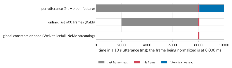
The released models agree with their recipes. Reading the preprocessor settings out of the model files themselves (code/ch02_features/results/model_frontends.json): the offline Parakeet CTC 0.6B model says per_feature; both streaming models, the FastConformer and Nemotron 3.5 ASR, say NA. The per-utterance normalization row of the WER table above shows what happens when you apply the offline habit to a streaming model anyway.

How much does the future move the past? I kept the first second of one utterance fixed and changed only what came after it (code/ch02_features/results/normalization_leak.json). With per-utterance mean and variance normalization, replacing the rest of the utterance by 4 s of silence changed the features of that first second by 2.13 on average; replacing it by loud noise, by 1.28. With a running (causal) normalizer, a 600-frame window or none, the change was exactly 0. The first second's audio was the same in every case. Only its features moved.

Whisper's front end reads its window

Whisper is a special case worth knowing because it is often wrapped for streaming (chapter 8). Its features are log10 of power, then clamped to at most 8 below the largest value, then rescaled: log_spec = torch.maximum(log_spec, log_spec.max() - 8.0) and (log_spec + 4.0) / 4.0 (whisper/audio.py, lines 154-156). The maximum is taken over the whole input, which Whisper always pads or trims to 30 s (3,000 frames). So every feature value depends on the loudest moment anywhere in that window, including moments after it. The paper describes the scaling as global over the training set (arXiv:2212.04356, p. 3); the code, which is what the released models run, does this per input.

Common misconceptions

"An 80-bin log-mel is a standard feature." It is a recipe with at least ten settings, and the eight front ends above disagree on most of them. Read the front end out of the model's own files.

"Features are computed from the samples the model has received." Each frame needs audio past its own hop: 7.5 ms with the CPU track's framing, 15 ms with Kaldi's default. A streaming front end holds the last partial window back until the next chunk arrives.

"The spectrum of one frame tells you the word." One frame is 25 ms, shorter than most speech sounds, and it holds no time order. It tells you a vowel's formants or that a sound is a hiss, not which word is being said. The words are in how the spectra change over many frames, which is what the model's layers read.

Try it

The scripts are in code/ch02_features/; setup is in code/README.md.

CPU track

1. python code/ch02_features/frontend_compare.py computes the 80-bin log-mel of one utterance with three implementations and with one option changed at a time. Check that the three implementations agree to about 0.0001 and that the int16-scale row shows an offset of 20.79.
2. python code/ch02_features/normalization_leak.py runs the "change only the future" test. Every normalizer that is safe for streaming must print 0.
3. python code/ch02_features/model_frontends.py reads the preprocessor block out of each NeMo model file without loading the model, and prints sherpa-onnx's defaults. Find normalize in each.
4. python code/ch02_features/dft_by_hand.py computes the 8-point transform of the Fourier section with a loop and writes results/dft_by_hand.json. Expect samples 5, 6, −3, −1, −5, −6, 3, 1; magnitudes 19.928 in bin 1 and 13.071 in bin 3, 0 elsewhere in bins 0 to 4; and max_abs_difference_to_numpy_fft below 1e-10. Change the samples and predict the bins before you run it.
5. python code/ch02_features/read_spectrogram.py measures the marked ranges of the two spectrograms and writes results/read_spectrogram.json. Expect f0_hz 93.4 and formants 589, 970 and 2,541 Hz for the English vowel, a falling f0 (254.3 to 228.5 Hz) and a rising f0 (214.6 to 247.0 Hz) for the two Mandarin tones. Then change a time range in SEGMENTS by 0.1 s and see which numbers move.
6. python code/ch02_features/mel_numbers.py writes results/mel_numbers.json. Expect 28, 34 and 18 filter centers in the three bands, a loudest-to-quietest frame ratio of 139,332 (11.845 in natural-log units) and a mean log change of −1.3863 for the halved signal.

The data for the new figures is exported by figures/ch02/data/export_dft_by_hand.py and figures/ch02/data/export_read_spectrogram.py.

GPU track

code/ch02_features/frontend_mismatch_nemo.py produced the WER table above. It is in the GPU track because it needs the GPU track's ssh-nemo environment, but it runs on a CPU (CUDA_VISIBLE_DEVICES= python code/ch02_features/frontend_mismatch_nemo.py). Add your own mistake as a seventh variant: for example, features computed with torchaudio's MelSpectrogram defaults.

English and Mandarin

The front end is the same for both languages: nothing in this chapter depends on the words. To see it, run step 1 with a Mandarin utterance from code/data/manifests/aishell1-test-200.tsv (the manifests store paths relative to $BOOK_DATASETS; prefix them with it) by changing WAV at the top of the script, and an output path of your own so the English result file is kept. Check that the three implementations agree as closely as they did on the English utterance.

Key terms

• discrete Fourier transform (DFT): N samples in, N numbers out, one per bin; bin k measures how much of the signal repeats k times in the N samples. The FFT is its fast algorithm.
• bin: one output of the transform; its frequency is k times the sample rate divided by N.
• magnitude: the length of a bin's complex value; how much of that frequency is present, without the phase.
• harmonic: a multiple of the voice's pitch; a voiced sound has energy at f0, 2 f0, 3 f0 and so on.
• formant: a broad hump of energy shaped by the throat and mouth; the first two or three tell vowels apart.
• fricative: a consonant made by forcing air through a narrow gap (s, sh, f; z and v when voiced); noise spread over high frequencies, with a buzz at low frequencies added when voiced.
• stop release (burst): the click when a closed mouth opens (p, t, k, b, d, g); a short vertical stripe. An affricate (zh, j, ch) is a stop release followed by a fricative.
• spectral centroid: the power-weighted average frequency of a sound.
• mel scale: a frequency scale that is finer at low frequencies, built to follow hearing.
• MFCC: log-mel values followed by a discrete cosine transform, keeping the first few outputs.
• frame: one short slice of audio for feature extraction, usually 25 ms.
• window: the taper multiplied into a frame (Hann, povey), and also its length.
• hop: the distance between the starts of consecutive frames, usually 10 ms.
• snip_edges: Kaldi's choice between frames that fit inside the audio and frames centered on their hop.
• spectrogram: power per frequency bin per frame.
• mel filterbank: triangular filters spaced on a mel scale (HTK or Slaney) that pool the spectrum.
• log-mel feature / fbank: the logarithm of each mel filter's output; what the models read.
• CMVN: subtracting a mean and dividing by a standard deviation per feature dimension.
• per-utterance normalization: CMVN with statistics of the whole utterance; reads the future.

Sources

• Kaldi (commit e02e35f): src/doc/feat.dox, src/feat/feature-window.{h,cc}, src/feat/feature-fbank.h, src/feat/mel-computations.h, src/feat/online-feature.h (and src/doc/feat.dox lines 68-72 for MFCC): https://github.com/kaldi-asr/kaldi/tree/e02e35f0254bb033fab73d1df99fc34123e31d56
• torchaudio (commit 9b19155): src/torchaudio/compliance/kaldi.py, src/torchaudio/transforms/_transforms.py: https://github.com/pytorch/audio/tree/9b19155e6fce04a83704eadc85d3dfe99e520c0c
• lhotse (commit 516c59b): lhotse/features/kaldi/extractors.py: https://github.com/lhotse-speech/lhotse/tree/516c59b3953132361fbd17c5976f07fa147381b4
• icefall (commit 9c96676): egs/librispeech/ASR/local/compute_fbank_librispeech.py, egs/librispeech/ASR/zipformer/streaming_decode.py: https://github.com/k2-fsa/icefall/tree/9c966762e058bd7ba79d9da71e42fc06b64b703e
• sherpa-onnx (commit 935e5de): sherpa-onnx/csrc/features.h: https://github.com/k2-fsa/sherpa-onnx/tree/935e5ded3d949a8b557ac44ef4dad03a7d2038e7
• kaldi-native-fbank (commit a8d31aa): kaldi-native-fbank/csrc/feature-window.h, feature-fbank.h: https://github.com/csukuangfj/kaldi-native-fbank/tree/a8d31aa6a06fb93b69925b23c3bd17d95338b6dd
• NeMo (commit 8eb458b): nemo/collections/asr/parts/preprocessing/features.py, nemo/collections/asr/modules/audio_preprocessing.py, examples/asr/conf/fastconformer/cache_aware_streaming/fastconformer_transducer_bpe_streaming.yaml: https://github.com/NVIDIA/NeMo/tree/8eb458b8ee304143426be5070d3f55fb3b5fb736
• WeNet (commit be6ad97): wenet/models/transformer/cmvn.py: https://github.com/wenet-e2e/wenet/tree/be6ad97fdb512589df113042f7ff3a29d392fb38
• openai/whisper (commit 8609812): whisper/audio.py: https://github.com/openai/whisper/tree/86098128c0b4f24f0e2aa2994de830614b474227
• Radford et al., "Robust Speech Recognition via Large-Scale Weak Supervision", arXiv:2212.04356 (Sec. 2.2: the 80-channel log-magnitude Mel spectrogram).
• librosa 0.11.0: librosa/core/spectrum.py, librosa/core/convert.py, librosa/feature/spectral.py: https://github.com/librosa/librosa/tree/0.11.0
• Hugging Face Audio Course, Unit 1 (commit 56b6e83): https://github.com/huggingface/audio-transformers-course/tree/56b6e8334aef7e0efa0137574f068c968f3f6e1c