4. From offline to streaming ASR: CTC, transducer, attention

What you will learn

• The problem every speech recognizer has to solve: audio has many more frames than the text has letters, and nobody tells the model which frame belongs to which letter.
• How the three families of end-to-end recognizers solve it: CTC, the transducer (RNN-T) and attention encoder-decoders (AED).
• How to compute the CTC and transducer probabilities by hand for a tiny example, so that the losses stop being black boxes.
• Why CTC and transducers stream naturally and attention models do not, and which variants make transducers cheaper and faster.

Before you start

• Chapters: 1-3. You need the idea of a feature frame (chapter 2: one every 10 ms) and of an encoder that turns frames into a shorter sequence of vectors (here, one vector every 40 or 80 ms).
• Tools: Python with numpy and torch for the exercises; no GPU.

The alignment problem

A recognizer reads a sequence of encoder frames, say 25 frames for a second of speech at 40 ms per frame, and must produce a sequence of output units: letters, subword pieces or Chinese characters, say 12 of them. The training data gives you the audio and the text, but not which frame each unit belongs to. That missing information is the alignment.

Older systems got alignments from a separate model and trained frame by frame. End-to-end models avoid that by summing over all alignments that are consistent with the text. The three families differ in what an alignment is and how the sum is computed, and that difference decides whether they can stream.

CTC: one output per frame, with a blank

Connectionist temporal classification (CTC) (Graves et al., ICML 2006, PDF) gives the network one output distribution per frame, over the labels plus one extra symbol, the blank: "A CTC network has a softmax output layer ... with one more unit than there are labels in L. ... The activation of the extra unit is the probability of observing a 'blank', or no label" (Sec. 3.1, p. 2).

A path is one symbol per frame. Its probability is the product of the per-frame outputs, p(π|x) = ∏t y^t (Eq. 2), which assumes "that the network outputs at different times are conditionally independent, given the internal state of the network" (p. 3).

A path becomes a labelling by the collapse rule B: first merge repeated symbols, then remove blanks. Graves' own example: B(a−ab−) = B(−aa−−abb) = aab (Sec. 3.1, p. 3). The blank between two a's is what lets "aa" survive; without it, the two would merge into one. The probability of a labelling is the sum over all paths that collapse to it (Eq. 3):

p(l | x) = Σ_{π ∈ B⁻¹(l)} p(π | x)

The CTC loss for one example is −ln p(l | x) for its reference transcript; Eq. 12 sums this over the training set.

Computing it by hand

Take three frames, the alphabet {a, b} plus blank (written −), and the target "ab". Suppose the network outputs these per-frame probabilities (made up for the example):

frame	−	a	b
t = 1	0.5	0.4	0.1
t = 2	0.3	0.3	0.4
t = 3	0.6	0.1	0.3

Of the 3³ = 27 possible paths, five collapse to "ab":

path	probability
− a b	0.5 · 0.3 · 0.3 = 0.045
a − b	0.4 · 0.3 · 0.3 = 0.036
a a b	0.4 · 0.3 · 0.3 = 0.036
a b −	0.4 · 0.4 · 0.6 = 0.096
a b b	0.4 · 0.4 · 0.3 = 0.048
sum	p(ab | x) = 0.261

So the loss is −ln 0.261 = 1.343.

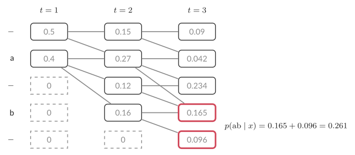
Enumerating paths is fine for three frames and hopeless for three hundred. The forward algorithm computes the same sum in time proportional to frames × labels. Write the target with blanks around and between the labels: l' = (−, a, −, b, −), five positions. Let α_t(s) be the total probability of all path prefixes of length t that end at position s of l' and are consistent with the target so far (Graves 2006, Eq. 5). Start with α_1(1) = y^1_− and α_1(2) = y^1_a; every other α_1 is 0. Then each step allows three moves into position s: stay at s, come from s − 1, or skip from s − 2, and the skip is allowed only when it jumps over a blank between two different labels (Eqs. 6-7). Multiply by the probability of l'_s at frame t:

t	α(1) −	α(2) a	α(3) −	α(4) b	α(5) −
1	0.5	0.4	0	0	0
2	0.15	0.27	0.12	0.16	0
3	0.09	0.042	0.234	0.165	0.096

Three cells worked out:

• α_2(4) = (α_1(4) + α_1(3) + α_1(2)) · y^2_b = (0 + 0 + 0.4) · 0.4 = 0.16. The skip from a to b over the blank is allowed because a ≠ b.
• α_3(3) = (α_2(3) + α_2(2)) · y^3_− = (0.12 + 0.27) · 0.6 = 0.234. No skip into a blank.
• α_3(4) = (α_2(4) + α_2(3) + α_2(2)) · y^3_b = (0.16 + 0.12 + 0.27) · 0.3 = 0.165.

A complete path must end on the last label or the final blank, so p(ab | x) = α_3(5) + α_3(4) = 0.096 + 0.165 = 0.261 (Eq. 8), the same as the enumeration. torch.nn.functional.ctc_loss on these numbers returns 1.343.

Greedy decoding and its trap

At inference time the simplest decoder takes the most probable symbol at every frame and collapses the result. Graves calls it best-path decoding: "trivial to compute ... However it is not guaranteed to find the most probable labelling" (Sec. 3.2, p. 3). The reason is that many paths add up to one labelling. Two frames over the alphabet {a} make the point. Let each frame give blank 0.6 and a 0.4. The best path is "− −" (0.36), which collapses to the empty string. But the labelling "a" collects three paths, "a −", "− a" and "a a", for 0.24 + 0.24 + 0.16 = 0.64. Greedy decoding returns nothing; the most probable answer is "a". In practice CTC outputs are peaky (one confident frame per label and blank elsewhere), so greedy decoding is usually close; beam search, in chapter 6, closes the rest of the gap.

What CTC cannot do

The conditional independence in Eq. 2 is also CTC's weakness. Each frame's output ignores what was output at the other frames, so CTC has no built-in model of the output language. And a labelling can be no longer than the number of frames: "as well as precluding tasks, such as text-to-speech, where the output sequence is longer than the input sequence, CTC does not model the interdependencies between the outputs" (Graves 2012, arXiv:1211.3711, Sec. 1).

For streaming, CTC has a decisive strength: frame t's output depends only on the encoder vector at frame t. If the encoder streams, so does the recognizer.

The transducer: emit labels, or move on

The transducer, introduced as the RNN transducer or RNN-T (Graves 2012), keeps CTC's "output nothing" symbol, written ∅, but changes what an alignment is. At each encoder frame the model can emit any number of labels before it moves to the next frame. An alignment is a sequence of label emissions and ∅ symbols; removing the ∅'s gives the transcript (Eq. 1). "The intuitive meaning of ∅ is 'output nothing'" (Sec. 2, p. 2).

Two networks produce the probabilities:

• the encoder (Graves calls it the transcription network) turns the audio into vectors f_1 ... f_T;
• the prediction network reads the labels emitted so far and produces vectors g_0 ... g_U, one per label prefix.

A small joiner combines f_t and g_u into a distribution over the labels plus ∅. In the original paper the combination is additive, h(k, t, u) = exp(f_t^k + g_u^k), normalized over k (Eqs. 12-13). Because the prediction network sees the previous labels, the transducer, unlike CTC, models dependencies between outputs.

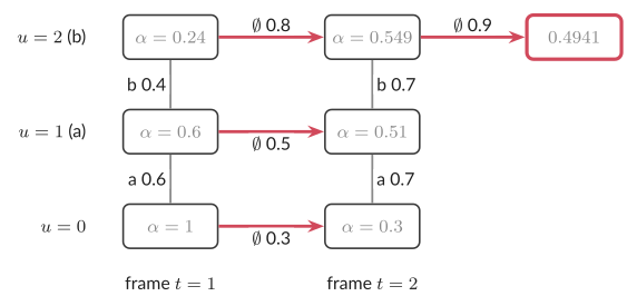
The probabilities live on a lattice of nodes (t, u): "the horizontal arrow leaving node t, u represents the probability ∅(t,u) of outputting nothing at (t,u); the vertical arrow represents the probability y(t,u) of outputting the element u+1 of y" (Fig. 1 caption, p. 4). Every alignment is a staircase from (1, 0) to (T, U) that ends with a ∅ at the last frame.

Computing it by hand

Take two encoder frames and the target "ab" (U = 2). The only probabilities needed are ∅(t, u) and the probability of the next label at each node:

node (t, u)	∅(t, u)	next label y(t, u)
(1, 0)	0.3	P(a) = 0.6
(1, 1)	0.5	P(b) = 0.4
(1, 2)	0.8	—
(2, 0)	0.2	P(a) = 0.7
(2, 1)	0.2	P(b) = 0.7
(2, 2)	0.9	—

The forward variable α(t, u) is the probability of reaching node (t, u). It obeys α(t, u) = α(t − 1, u) · ∅(t − 1, u) + α(t, u − 1) · y(t, u − 1), with α(1, 0) = 1 (Eq. 16):

• α(1, 1) = 1 · 0.6 = 0.6; α(1, 2) = 0.6 · 0.4 = 0.24; α(2, 0) = 1 · 0.3 = 0.3
• α(2, 1) = α(1, 1) · ∅(1, 1) + α(2, 0) · y(2, 0) = 0.6 · 0.5 + 0.3 · 0.7 = 0.51
• α(2, 2) = α(1, 2) · ∅(1, 2) + α(2, 1) · y(2, 1) = 0.24 · 0.8 + 0.51 · 0.7 = 0.549

The total is P(ab | x) = α(2, 2) · ∅(2, 2) = 0.549 · 0.9 = 0.4941 (Eq. 17), and the loss is −ln 0.4941 = 0.705.

There are three alignments, because an alignment has exactly T = 2 ∅'s and U = 2 labels and ends in ∅, so the labels go in two of the first three slots:

• ∅ a b ∅ (both labels at frame 2): 0.3 · 0.7 · 0.7 · 0.9 = 0.1323
• a ∅ b ∅ (a at frame 1, b at frame 2): 0.6 · 0.5 · 0.7 · 0.9 = 0.1890
• a b ∅ ∅ (both labels at frame 1): 0.6 · 0.4 · 0.8 · 0.9 = 0.1728

They sum to 0.4941. Notice what distinguishes them: not which labels, but when each label is emitted. A model trained only to maximize this sum has no reason to prefer early emission over late. That freedom is the root of the transducer's emission delay, which chapter 6 measures and corrects.

Why it streams

The joiner at (t, u) needs only f_t and g_u. The prediction network runs on labels already emitted. So once the encoder streams (the subject of chapter 5), the transducer decodes as audio arrives, one frame at a time. Graves' 2012 model used a bidirectional encoder, which does not stream; the streaming property comes from replacing it with a causal or chunked one. Google's on-device RNN-T, an early production example, "can outperform a conventional CTC-based model in terms of both latency and accuracy in a number of evaluation categories" (arXiv:1811.06621, abstract).

Making transducers cheap enough

The joiner produces a distribution over the whole vocabulary at every (t, u) node, so training holds a tensor of size batch × T × U × V. With thousands of Chinese characters as V, that is the bottleneck, which is exactly the case the pruned RNN-T addresses ("For large vocabulary sizes (e.g. Chinese characters)...", arXiv:2206.13236, Sec. 1). It first runs a cheap "trivial joiner" to find, for each frame, the few label positions that matter, then evaluates the full joiner only at "a constant S, e.g. S = 4 or S = 5" of them (Sec. 3.2). On one V100, LibriSpeech-shaped batches of 30 took 64 ms and 3.73 GB, against 544 ms and 18.48 GB for torchaudio's full loss (Table 1), at the same accuracy as a model trained with the optimized_transducer loss (2.56/6.27% against 2.61/6.46% WER on test-clean/test-other, Table 3).

Two other changes appear in the models you will run:

• Stateless prediction network. The k2/icefall recipes replace the LSTM prediction network with "an embedding layer followed by a 1-D convolutional layer with a kernel size 2" (arXiv:2206.13236, Sec. 4.2): the network sees only the last two labels (--context-size 2, icefall egs/librispeech/ASR/zipformer/train.py lines 419-423 at commit 9c96676). A related Google design shrank a decoder from 23M to 2M parameters at equal WER, but only after an extra training stage (EMBR); before it, WER was 6.4% against 6.1% (arXiv:2109.07513, Table 2).
• Token-and-duration transducer (TDT). NVIDIA's TDT predicts a token and how many frames to skip, from two separately normalized heads, P(v, d | t, u) = P_T(v | t, u) · P_D(d | t, u) (arXiv:2304.06795, Eq. 5). Skipping frames speeds up decoding: with non-batched greedy search, 1.9 to 2.2 times faster on LibriSpeech at equal WER, and up to 2.82 times on German Multilingual LibriSpeech (Tables 1-4).

Attention encoder-decoders: powerful, but they look at everything

An attention encoder-decoder (AED) generates the transcript one token at a time, like a language model, and at each step attends over the entire encoder output to decide where to look. Whisper is the best-known example. There is no blank and no explicit alignment; attention learns where to look.

That is exactly why it does not stream. To emit the first token, standard ("soft") attention reads all encoder frames, so the whole utterance must be heard first, and the cost grows with the square of the length: its "decoding process incurs a quadratic time and space cost and is inapplicable to real-time sequence transduction" (MoChA, arXiv:1712.05382, abstract). Attention is also free to look anywhere, which made early models "too flexible to predict proper alignments ... due to the lack of left-to-right constraints as used in CTC" (arXiv:1609.06773, abstract), the motivation for training CTC and attention jointly.

Chapter 5 shows the two ways attention models are made to stream anyway: restrict attention to chunks of audio, or use a streaming CTC or transducer for partial results and the attention decoder only to rescore at the end ("two-pass"). Chapter 8 covers wrappers that stream Whisper without retraining it.

The three families side by side

	CTC	transducer	attention encoder-decoder
alignment	one symbol per frame, collapse repeats and blanks	label emissions and ∅ on a frames × labels lattice	none; attention chooses where to look
models output dependencies	no	yes (prediction network)	yes (decoder)
streams when the encoder streams	yes	yes	no; needs chunked attention or two-pass
main cost	cheap	joiner over frames × labels × vocabulary	attention over all frames
typical use in this book	first-pass and lightweight recognizers	the streaming models of chapters 5-6, 9 and 15	rescoring and Whisper (chapter 8)

For a survey of all of them, Prabhavalkar et al. (arXiv:2303.03329, IEEE/ACM TASLP) is the place to start: its "goal ... is to provide a taxonomy of E2E ASR models".

Common misconceptions

"Greedy CTC decoding returns the most probable transcript." It returns the labelling of the most probable path. A labelling sums many paths, and in the two-frame example above the best path gives the empty string while the best labelling is "a".

"The transducer is streaming by design." The output layer is; the encoder may not be. Graves' original transducer used a bidirectional encoder. A transducer streams only with a causal or chunked encoder (chapter 5).

"A transducer emits a label as soon as it has heard it." The loss sums over all alignments and does not care when labels are emitted. Trained naively, transducers learn to wait for more context and emit late. Chapter 6 shows how FastEmit and the delay penalty push emission earlier.

Try it

The scripts are in code/ch04_alignment/ (environment ssh-asr, see code/README.md). They need only a CPU.

CPU track

1. python code/ch04_alignment/chapter_examples.py recomputes both hand-worked examples of this chapter. For CTC, the five enumerated paths sum to 0.261, and the loss is 1.3432 three ways: from the enumeration, from the numpy forward algorithm in code/hbasr/alignment.py, and from torch.nn.functional.ctc_loss. For the transducer, the forward table is α(1, ·) = 1, 0.6, 0.24 and α(2, ·) = 0.3, 0.51, 0.549, the total 0.4941, and the loss 0.7050 by hand and from torchaudio.functional.rnnt_loss (which runs in float32, so it agrees to six digits). Change one probability in the script and predict the new α table before you run it.
2. Lower ∅(1, 1) from 0.5 to 0.1 in the transducer example. Which of the three alignments loses probability, and does the total go up or down? (In the script, the probability ∅(1, 1) gives up goes to the label a, which no alignment of "ab" uses at that node.)
3. python code/ch04_alignment/ctc_rnnt_by_hand.py enumerates every alignment for a few more examples, including random distributions over 6 frames, and checks the forward algorithm against PyTorch for each. Use it to count alignments: for T frames and U labels, check C(T + U − 1, U) for the transducer against the enumeration, and count CTC paths for the same target.

GPU track

Nothing in this chapter needs a GPU; chapter 5 runs the streaming encoders.

English and Mandarin

The vocabulary decides the transducer's cost. The joiner computes a distribution over the whole vocabulary at every node of the lattice, T × (U + 1) nodes. For the two CPU-track models and one test utterance each, computed by chapter_examples.py from the models' own tokens.txt and bpe.model:

Model	Utterance	Output symbols V	Tokens U	Encoder frames T (40 ms)	Joiner values T × (U + 1) × V
English Zipformer (BPE)	LibriSpeech 1089-134686-0006, 10.6 s	502	53	264	7.2 million, 28.6 MB in fp32
Mandarin Zipformer (characters + BPE)	AISHELL-1 BAC009S0764W0140, 6.2 s	2,002	18	155	5.9 million, 23.6 MB in fp32

A Mandarin utterance has fewer tokens, because most characters are one token (rarer ones are spelled as byte tokens, which is why 16 characters became 18 tokens here), but four times as many symbols to score at each node. Per utterance this is fine; in training, with a batch of long utterances, the full joiner output is what runs out of memory, which is why pruned RNN-T (above) exists.

Key terms

• alignment: which frame each output unit belongs to.
• blank (CTC), ∅ (transducer): the extra symbol meaning "output nothing here".
• path (CTC): one symbol per frame; collapsing it gives a labelling.
• collapse rule: merge repeated symbols, then remove blanks.
• forward algorithm: dynamic programming that sums the probability of all alignments.
• transducer (RNN-T): encoder, prediction network and joiner on a frames × labels lattice.
• prediction network: the part of a transducer that reads previously emitted labels.
• joiner: combines encoder and prediction vectors into a distribution over labels and ∅.
• attention encoder-decoder (AED): a decoder that generates tokens while attending over all encoder frames.
• emission delay: how late, relative to the audio, a model emits each label.

Sources

• Graves, Fernández, Gomez, Schmidhuber, Connectionist Temporal Classification, ICML 2006, doi:10.1145/1143844.1143891: https://www.cs.toronto.edu/~graves/icml_2006.pdf
• Graves, Sequence Transduction with Recurrent Neural Networks, arXiv:1211.3711 (2012): https://arxiv.org/abs/1211.3711
• Kuang et al., Pruned RNN-T for fast, memory-efficient ASR training, arXiv:2206.13236: https://arxiv.org/abs/2206.13236
• Botros et al., Tied & Reduced RNN-T Decoder, arXiv:2109.07513: https://arxiv.org/abs/2109.07513
• Xu et al., Efficient Sequence Transduction by Jointly Predicting Tokens and Durations (TDT), arXiv:2304.06795: https://arxiv.org/abs/2304.06795
• Monotonic Chunkwise Attention, arXiv:1712.05382: https://arxiv.org/abs/1712.05382
• Joint CTC-Attention based End-to-End Speech Recognition using Multi-task Learning, arXiv:1609.06773: https://arxiv.org/abs/1609.06773
• Streaming End-to-end Speech Recognition For Mobile Devices, arXiv:1811.06621: https://arxiv.org/abs/1811.06621
• Prabhavalkar et al., End-to-End Speech Recognition: A Survey, arXiv:2303.03329: https://arxiv.org/abs/2303.03329
• icefall, commit 9c96676: https://github.com/k2-fsa/icefall/tree/9c966762e058bd7ba79d9da71e42fc06b64b703e