3. The vocabulary of latency

What you will learn

• The parts that "latency" splits into in a streaming speech system: look-ahead, compute, emission delay, endpoint delay and, for speech synthesis, time to first audio.
• Why a model that runs ten times faster than real time can still feel slow, and what real-time factor does and does not tell you.
• How to read a streaming configuration such as NeMo's att_context_size [70,13] as three different millisecond numbers.
• How many requests a percentile needs before you should believe it.

Before you start

• Chapters: 1 and 2 (samples, chunks, 10 ms feature frames, the front end's few milliseconds of look-ahead).
• Tools: the ssh-asr environment from code/README.md. Everything in Try it runs on a CPU.

One utterance, measured

Start with a measurement and name its parts afterwards. I streamed one LibriSpeech test-clean utterance (10.6 s, 24 words) into the CPU track's streaming recognizer, a Zipformer transducer (chapters 4 and 5 explain both words; sherpa-onnx, one thread, model chunk 320 ms), sending it in 160 ms chunks at the pace a microphone would deliver them. After each chunk the harness recorded the time and the text on screen (code/ch03_latency/results/harness_demo.json).

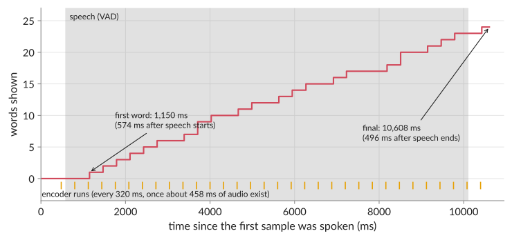
Read the figure from left to right.

• Speech starts at 576 ms (the first 576 ms are silence, found by a voice activity detector).
• The encoder runs for the first time when the chunk ending at 480 ms arrives, and from then on every 320 ms: every second 160 ms chunk. Each run took about 28 ms (median of 32 runs).
• The first word appears at 1,149 ms, 573 ms after speech starts.
• Speech ends at 10,112 ms. The audio file ends at 10,555 ms. The final result is ready at 10,608 ms: 53 ms after the audio ended, 496 ms after the speaker stopped.
• The whole utterance cost 0.10 s of computation per second of audio.

These are five different numbers, and each answers a different question. The rest of the chapter names them.

Chunk and look-ahead

A streaming recognizer receives audio in chunks: here 160 ms, 2,560 samples. The chunk size the client sends and the chunk size the model processes need not be the same. This model processes 320 ms at a time, so it waits for two client chunks.

To process a chunk the model also needs some audio after it, its look-ahead. Chapter 2 found 7.5 ms of it in this model's front end. The Zipformer reads 13 feature frames, 130 ms, past each 320 ms chunk (the pad_length = 7 + 2 * 3 feature frames of icefall's streaming code, decode_stream.py, line 79). So its first run needs the 45th feature frame, which ends at sample 160 × 44 + 280 = 7,320: about 458 ms of audio (320 ms of chunk, 130 ms of feature look-ahead and the last window's 7.5 ms). In 160 ms chunks, that is available when the third chunk arrives, at 480 ms, which is exactly when the figure shows the first run.

Algorithmic latency is the delay these two cause even on an infinitely fast computer: "the time span that the audio chunk represents, along with any required look-ahead frames" (Shangguan et al. 2021, arXiv:2104.02207, Sec. 1). A sound at the start of a chunk waits for the rest of the chunk and the look-ahead; a sound at the end of it waits only for the look-ahead.

Reading att_context_size: three numbers for one setting

NVIDIA's cache-aware models, on the GPU track, describe their latency with a pair [left, right] counted in encoder frames, and a frame is 80 ms because the encoder subsamples 10 ms features by a factor of eight. The recipe's comment gives the formula: "look-ahead(secs) = att_context_size[1]*subsampling_factor*window_stride, example: 13*8*0.01=1.04s" (fastconformer_transducer_bpe_streaming.yaml, lines 104-114). In the code, a chunk is att_context_size[1] + 1 frames (conformer_encoder.py, lines 886-895). So the single setting [70,13] hides three numbers, and you will see all three quoted:

• Chunk: 1,120 ms. 14 frames of 80 ms. The Nemotron 3.5 ASR model card, whose setting is [56,13], quotes this one ("Chunk size = 14 (14 × 80ms = 1.12s)").
• Worst-case look-ahead: 1,040 ms. The first frame of a chunk waits for the 13 frames after it. The FastConformer model card quotes this one ("[70,13]-1040ms").
• Average look-ahead: 520 ms. The look-ahead "varies in the range 0, C −1", and "the average of latency for each case is half of the look-ahead size" (Noroozi et al., arXiv:2312.17279, Sec. 3.1 and Sec. 4).

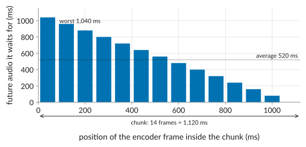
The left number, 70, is look-back: 70 frames, 5.6 s of past context the encoder keeps in a cache. It costs memory and compute, not waiting. The same arithmetic for the other trained settings:

att_context_size	Chunk	Worst look-ahead	Average look-ahead
[70,0]	80 ms	0 ms	0 ms
[70,1]	160 ms	80 ms	40 ms
[70,6]	560 ms	480 ms	240 ms
[70,13]	1,120 ms	1,040 ms	520 ms

Two traps. First, these milliseconds assume 8x subsampling; on a 4x model the same [70,13] means a 560 ms chunk and a 520 ms worst case. Second, the FastConformer card's usage text also lists [70,16] and [70,33]. NeMo rejects both: the left context must be a multiple of the chunk, and 70 is not a multiple of 17 or 34 (conformer_encoder.py, lines 983-985). The card's own result tables use [70,6] and [70,13], which hold.

Compute latency and real-time factor

The computer is not infinitely fast. Compute latency is the time the model takes to process a chunk once its audio is there: about 28 ms per 320 ms chunk in the measurement above.

The real-time factor (RTF) divides total processing time by the audio's duration: "the ratio of the time required to process audio frames relative to the length of the audio" (arXiv:2104.02207, Sec. 3.2). The utterance above had an RTF of 0.10. Smaller is faster; below 1 the system keeps up with a live speaker. Leaderboards often print the inverse, RTFx = audio duration / processing time, so that higher is better: the Open ASR Leaderboard defines it that way and measures it over batches of up to 64 utterances (arXiv:2510.06961, Secs. 2 and 3). An RTF of 0.10 is an RTFx of about 10.

RTF is a throughput number. It says nothing about when the words appear, as one experiment shows clearly. Shangguan et al. compared two models of their Table 1, the second 55% cheaper (26.3 M against 11.8 M FLOPS) with half the RTF (0.42 against 0.21), and the median user-perceived latency was 2% worse, 1.47 s to 1.50 s (arXiv:2104.02207, Table 1). As long as RTF stays below 1, the time a user waits is set by look-ahead and endpointing, not by how fast the model runs; the same paper notes that "for models with RTF≥1, the decoder catchup lag becomes significant".

A second measurement makes the point from the other side. With real-time pacing and with simulated pacing (feeding chunks as fast as the CPU can take them, with a virtual clock), the harness produced the same partial results after every chunk and the same final text. Pacing changes when the work happens, not what the model computes. That is why the harness in this book can measure latency without sleeping.

Emission delay and first-token delay

Even when a chunk has been processed, the model may not yet output the word it contains. Streaming models learn to wait for more context before committing to a token. Emission delay is the time from when a word was spoken to when the recognizer outputs it. Chapter 6 shows how training penalties push it down.

You cannot measure it from the text alone: you need to know when each word was spoken. Without word timings, two simpler numbers are used:

• First-token delay: "the time between when the user actually begins speaking (i.e., ignoring any initial silence) and the time when the ASR system actually emits an output token" (arXiv:2104.02207, Sec. 2). Above: 573 ms.
• Partial delay: for each word, the time until it first appears on screen after the start of the utterance, averaged (Shangguan et al. 2020, arXiv:2006.01416, Sec. 5.1).

A configured look-ahead is a lower bound on these, not an estimate of them. A 2026 paper on training streaming recognizers measured Voxtral Realtime at its 80 ms setting and found a median word-level emission delay of 0.77 s, "nearly an order of magnitude above the nominal 80 ms" (arXiv:2609.18333, Sec. 1). Measure it; do not read it off the configuration.

Endpoint delay and user-perceived latency

In a conversation, what the user waits for is the end: when does the system decide they have finished and act on what they said? In this book the endpoint delay is the time from the end of speech to the system's decision that the user has finished. Shangguan et al. call the same span the user-perceived latency (UPL): "the time between when the user finishes speaking and the decision is made to close the microphone" (arXiv:2104.02207, Sec. 2). They split it into two factors: the "endpointer lag", "the time required by the endpointer to determine that the user is done speaking", and the "decoder catchup lag", the time to finish processing audio that arrived after speech ended.

The endpointer usually dominates. In the same paper, one model's median endpointer lag was 1.00 s and its median UPL 1.60 s (Table 2; the medians come from different distributions and need not add up), and the authors write that "EP lag is almost ≥ 50% of the overall UPL". The reason is simple: an endpointer waits for silence long enough to be sure the speaker is not just pausing. sherpa-onnx's default rule fires after 1.2 s of trailing silence once something has been decoded (rule2{true, 1.2, 0}, endpoint.h, lines 41-52). That is 2.6 times the 458 ms the model itself needs for a chunk and its look-ahead. Chapter 7 is about making this number smaller.

In the measurement above, endpointing was off and the end of the file stood in for it: the final result came 53 ms after the file ended, but 496 ms after the speaker stopped, because the file contains 443 ms of trailing silence. Which end point a number is measured from changes it by an order of magnitude. State it with every latency you report.

In a voice agent, the user's wait ends even later: when they hear the first audio of the reply. This book uses UPL for that whole span when it discusses the cascade (chapter 18), and always says which end point it means.

Time to first audio

Speech synthesis has its own first number. Time to first audio (TTFA) is, in this book, the time from when the text request arrives to when the first audible sample of the reply is available to play. The primary sources do not agree on a name or a definition. CosyVoice 2 calls it "first-package latency" and gives it as compute only: the language model's time for the first M tokens, plus one pass of flow matching and the vocoder (arXiv:2412.10117, Sec. 2.5). Moshi gives a "theoretical latency" of 160 ms, its 80 ms frame plus one step of acoustic delay, and "200ms in practice" (arXiv:2410.00037).

TTFA, like ASR latency, is set mostly by a chunk policy rather than by speed. FireRedTTS-1S reports two decoders on the same NVIDIA L20 card: one with an RTF of 0.1 and a first-packet time under 300 ms (an upper bound; the paper gives no percentile), and one that does three times as much work per second of audio, RTF 0.3, with a first-packet time under 150 ms (arXiv:2503.20499, abstract and pp. 4-5). The slower decoder starts speaking sooner because it emits audio in smaller pieces. Chapters 12 to 14 measure TTFA for the book's TTS models.

Percentiles and concurrency

One utterance gives one of each number. A service handles thousands, and the slow ones matter most: a user who waits 3 s once remembers it. So latencies are reported as percentiles: p50 (the median), p90, p95, p99. NVIDIA's Riva publishes its streaming latency exactly this way, as average, p50, p90, p95 and p99 for each number of concurrent streams, with audio sent at real-time pace (Riva ASR performance).

Two things decide whether a percentile can be trusted.

How many requests it came from. numpy's default percentile interpolates between sorted values at position (n − 1) × q (numpy _function_base_impl.py, v2.1.0). With 20 requests, the p95 sits at position 18.05, between the second-largest and the largest value. It is essentially "the second-worst request", and it moves whenever either of those does.

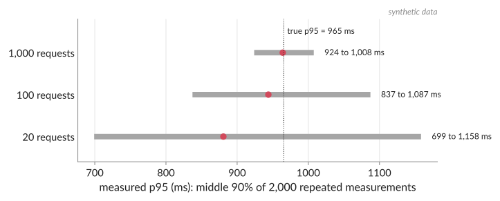
How many requests ran at once. A model that takes 30 ms per chunk alone may take far longer with 50 streams sharing a CPU or GPU. Latency without a concurrency level is not a property of a system, only of one load on it. Chapter 15 measures how latency grows with concurrency.

So every latency in this book comes with three labels: what it was measured from and to, at which percentile over how many requests, and at what concurrency.

Common misconceptions

"A model with RTF 0.1 answers in a tenth of the time." RTF is throughput. The model above had an RTF of 0.10 and still showed its first word 573 ms after speech started, because of chunking and look-ahead.

"The look-ahead setting is the latency." It is a lower bound for one frame. [70,13] alone is 1,120, 1,040 or 520 ms depending on what you count, and measured emission delay can be several times the configured look-ahead.

"Final latency is small, so the system is responsive." Measured from the end of the file, the final result above took 53 ms. Measured from the end of speech, 496 ms. With an endpointer, the end of speech is the honest starting point, and the endpointer's wait usually dominates.

Try it

CPU track

Run python code/ch03_latency/harness_demo.py (setup in code/README.md). It streams the utterance above into the English Zipformer twice, at real-time pace and with simulated pacing, and prints a line per chunk: audio time, when the chunk was processed, and the partial result. Check three things in its output:

1. The first chunk that triggers real work is the third one (ending at 480 ms). Change --chunk-ms to 100 and predict when the first run happens before you look (458 ms rounded up to whole 100 ms chunks).
2. Real-time and simulated pacing give the same partials and the same final text. Their RTFs are not the same: 0.096 and 0.074 in the run behind this chapter. Compute time varies from run to run; the outputs do not.
3. The last word of the utterance, "TAIL", is still "TA" after the last chunk and is completed only when the stream is closed. That is the look-ahead at work: the model needs audio after the word, and at the end of a stream there is none. So, as sherpa-onnx's own examples do, the harness appends 0.66 s of silence before it closes the stream: the exported model processes only whole chunks, and without the padding the last one would never fill. A client that only signals the end may never see "TAIL". The 53 ms of final latency above includes the computation on that padding.

The script also prints the att_context_size table for 4x and 8x subsampling. It includes [70,16] as an arithmetic example; NeMo will refuse to run it.

GPU track

None for this chapter. Chapter 9 runs the same harness on the GPU track's NeMo models.

English and Mandarin

Run the script again with --model zipformer-zh --wav <an AISHELL-1 test file> (paths in code/data/manifests/aishell1-test-200.tsv, relative to $BOOK_DATASETS). The Mandarin model uses the same chunk and look-ahead, so the first encoder run comes at the same moment; compare when the first character appears.

Key terms

• chunk: the piece of audio processed at once; the client's and the model's may differ.
• look-ahead: audio after a chunk that the model must wait for before processing it.
• algorithmic latency: chunk plus look-ahead; the delay on an infinitely fast computer.
• compute latency: the time to process a chunk once its audio has arrived.
• real-time factor (RTF): processing time divided by audio duration; RTFx is its inverse.
• emission delay: from when a word is spoken to when the recognizer outputs it.
• first-token delay: from the start of speech to the first output token.
• endpoint delay: from the end of speech to the decision that the user has finished.
• user-perceived latency (UPL): from the end of speech to the system's response; say which response.
• time to first audio (TTFA): from the text request to the first audible sample of synthesized speech.
• percentile (p50, p95, p99): the value below which that share of requests fall; needs a count.

Sources

• Shangguan et al., "Dissecting User-Perceived Latency of On-Device E2E Speech Recognition", arXiv:2104.02207.
• Shangguan et al., "Analyzing the Quality and Stability of a Streaming End-to-End On-Device Speech Recognizer", arXiv:2006.01416.
• Noroozi et al., "Stateful Conformer with Cache-based Inference for Streaming Automatic Speech Recognition", arXiv:2312.17279.
• "Open ASR Leaderboard: Towards Reproducible and Transparent Multilingual and Long-Form Speech Recognition Evaluation", arXiv:2510.06961.
• "Look Less, Hear Better: Jointly Rewarded GRPO for Streaming ASR", arXiv:2609.18333.
• Du et al., "CosyVoice 2: Scalable Streaming Speech Synthesis with Large Language Models", arXiv:2412.10117.
• Défossez et al., "Moshi: a speech-text foundation model for real-time dialogue", arXiv:2410.00037.
• "FireRedTTS-1S: An Upgraded Streamable Foundation Text-to-Speech System", arXiv:2503.20499.
• NeMo (commit 8eb458b): examples/asr/conf/fastconformer/cache_aware_streaming/fastconformer_transducer_bpe_streaming.yaml, nemo/collections/asr/modules/conformer_encoder.py: https://github.com/NVIDIA/NeMo/tree/8eb458b8ee304143426be5070d3f55fb3b5fb736
• NVIDIA model cards: nvidia/stt_en_fastconformer_hybrid_large_streaming_multi (revision ae98143), nvidia/nemotron-3.5-asr-streaming-0.6b (revision ea30d66), on Hugging Face.
• icefall (commit 9c96676): egs/librispeech/ASR/zipformer/decode_stream.py: https://github.com/k2-fsa/icefall/tree/9c966762e058bd7ba79d9da71e42fc06b64b703e
• sherpa-onnx (commit 935e5de): sherpa-onnx/csrc/endpoint.h: https://github.com/k2-fsa/sherpa-onnx/tree/935e5ded3d949a8b557ac44ef4dad03a7d2038e7
• NVIDIA Riva ASR performance page: https://docs.nvidia.com/deeplearning/riva/user-guide/docs/asr/asr-performance.html
• numpy v2.1.0: numpy/lib/_function_base_impl.py: https://github.com/numpy/numpy/tree/v2.1.0